SageMakerを使ってイメージ分類を、ラベル付け・訓練・推論まで一通り実行する
デープラーニングでイメージ分類を試していてGCP, Kubeflowなど検討したなかSageMakerが結構使いやすかったので、イメージ分類にどのように使用できるか紹介します。
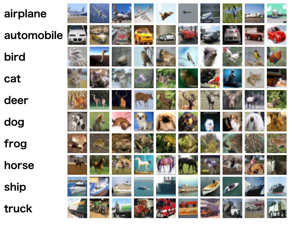
今回、CIFAR-10 dataset(Canadian Institute For Advanced Research)のデータセットを使って多クラスのイメージ分類を行います。CIFAR-10は以下のように1つのイメージが10クラス(airplane, automobile, bird, cat, deer, dog, frog, horse, ship, truck)のどれかに分類されるようなイメージがあつまったデータセットです。合計60,000枚のイメージが32x32ピクセルで保存されています。50,000枚が訓練データで、10,000枚がテストデータです。10クラスの分類なので1クラス6,000枚の画像があることになります。
今回使うSageMakerの機能
SageMakerの機能についてはAmazon Web ServicesブログでSageMakerを検索すると有益な情報がでてきます。とくにAWSの機械訓練サービス概要とAmazon SageMakerが有用です。
SageMakerにかかららず一般的な機械訓練ワークフローは以下のようになります(ここから引用)。
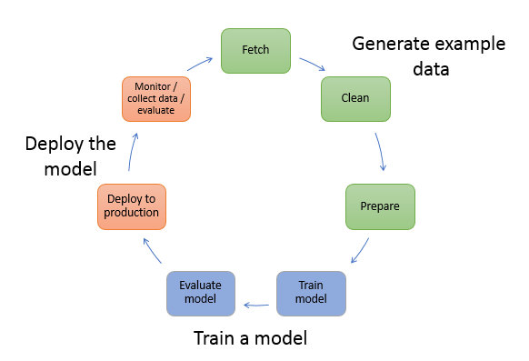
モデルを訓練するのはワークフローの一部でそれ以外に多くの作業があります。イメージ分類の場合、Generate example dataでは訓練させるためのイメージをあつめてそれに対してクラスをつけます。イメージも少量だと精度がでないので多く集めます。今回自分が関わっているところでは1クラスにつき1000枚ほどあつめています。Train a modelでは集めたイメージを分類させるためのモデルをTensorFlowやKerasなどを使って作ります。Deploy the modelでは作成したモデルをデプロイしてREST APIなどで未知のイメージに対して推論できるようにします。
SageMakerではこの機械訓練ワークフローのすべてに対応できる機能を備えています。SageMakerをAWSのWebコンソールで開くと以下のメニューがでてきます。
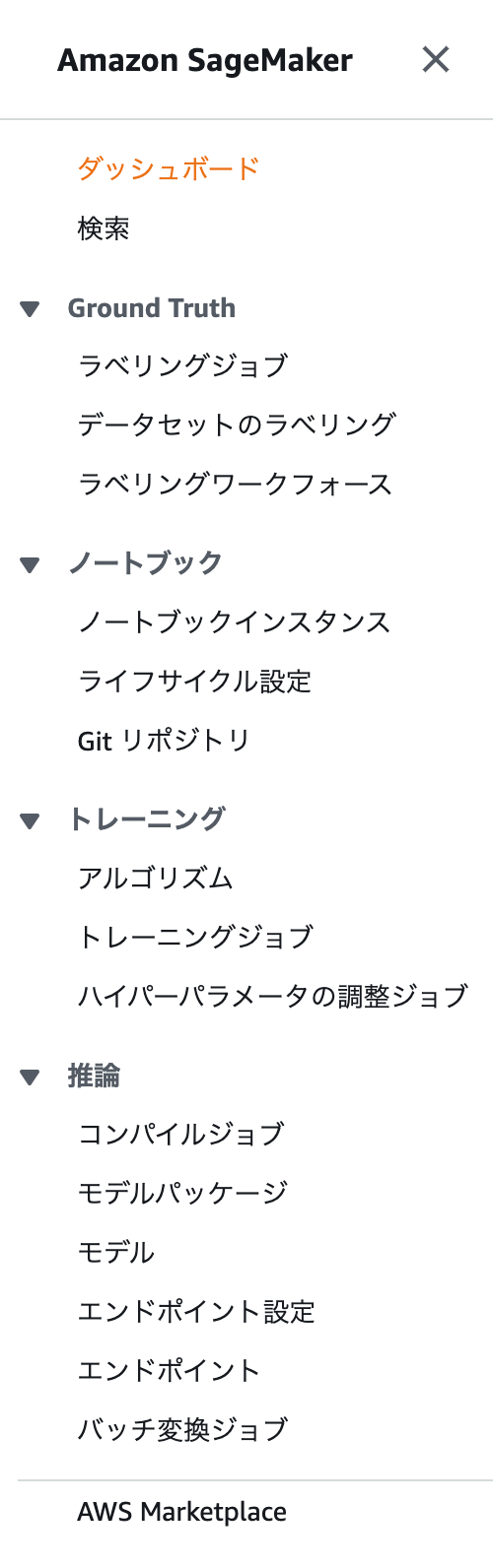
今回はSageMakerの機能だけを使って、以下のような作業でイメージ分類のモデルを作って、未知のイメージを推論できるまでを試します。
- 各種作業するためのノートブックを立ち上げる
- Ground Truthの機能でCIFAR-10のイメージにクラスを振る
- ノートブックでKerasを使ったモデルを構築しトレーニングジョブとして実行する
- 推論のエンドポイントを作成し、boto3から呼び出す
SageMakerでイメージ分類を行う
各種作業するためのノートブックを立ち上げる
SageMakerのノートブック > ノートブックインスタンスからJupyter Notebookのインスタンスを作成します。インスタンスサイズはなんでもいいですが今回はml.t2.mediumを選択しました。立ち上がったらOpen Jupyterでconda_tensorflow_p36のノートブックを立ち上げます。
ノートブックでCIFAR-10データセットをダウンロードしてS3にあげます。S3にあげるとGround Truthでクラスのラベリングができます。試しに100枚だけあげてみます(bucket_nameはバケットなので適切な値に変える必要があります)。
# 画像をダウンロードして展開
%%bash
wget https://www.cs.toronto.edu/~kriz/cifar-10-python.tar.gz
tar -xvf cifar-10-python.tar.gz
ls cifar-10-batches-py/

---
cifar-10-batches-py/
cifar-10-batches-py/data_batch_4
cifar-10-batches-py/readme.html
cifar-10-batches-py/test_batch
cifar-10-batches-py/data_batch_3
cifar-10-batches-py/batches.meta
cifar-10-batches-py/data_batch_2
cifar-10-batches-py/data_batch_5
cifar-10-batches-py/data_batch_1
import glob

def unpickle(file):
    import pickle
    with open(file, 'rb') as fo:
        dict = pickle.load(fo, encoding='latin-1')
    return dict

def output_data_to_png(input_data, root_dir):
    for i in range(len(input_data['filenames'])):
        filename = input_data['filenames'][i]
        data = input_data['data'][i]
        data = data.reshape(3, 32, 32)
        data = np.swapaxes(data, 0, 2)
        data = np.swapaxes(data, 0, 1)
        label_index = input_data['labels'][i]
        label_name = label_names[label_index]
        dirname = f"{root_dir}/{label_name}"
        if not os.path.exists(dirname):
            os.makedirs(dirname)
        with Image.fromarray(data) as img:
            img.save(f"{dirname}/{filename}")

meta_data = unpickle("cifar-10-batches-py/batches.meta")
label_names = meta_data['label_names']

files = [f for f in glob.glob("cifar-10-batches-py" + "**/test_*", recursive=True)]
for f in files:
    data = unpickle(f)
    output_data_to_png(data, "dataset/test")

files = [f for f in glob.glob("cifar-10-batches-py" + "**/data_*", recursive=True)]
for f in files:
    data = unpickle(f)
    output_data_to_png(data, "dataset/train")

!mkdir -p dataset/ground_truth/
for label in label_names:
    files = [f for f in glob.glob(f"dataset/train/{label}/*", recursive=True)]
    for f in files[:10]:
        !cp $f dataset/ground_truth/

!aws s3 cp --recursive dataset/ground_truth s3://bucket_name/cifar-10/dataset/ground_truth
Ground Truthの機能でCIFAR-10のイメージにクラスを振る
現実の問題でイメージ分類するときは教師データとしてイメージにクラスが割り振られている状態でなければいけません。Google Sheetで管理しながやるなり、内製でラベルをつけるWebサービスをつくるなりしなければならず結構手間です。SageMakerではGround Truthという機能で未分類のイメージに効率的にクラスをつけることができます。
CIFAR-10のイメージにはすでにクラスが割り振られていますが、Ground Truthを試したいので割り振られていない体でS3にあげたイメージをクラスに分類してみます。
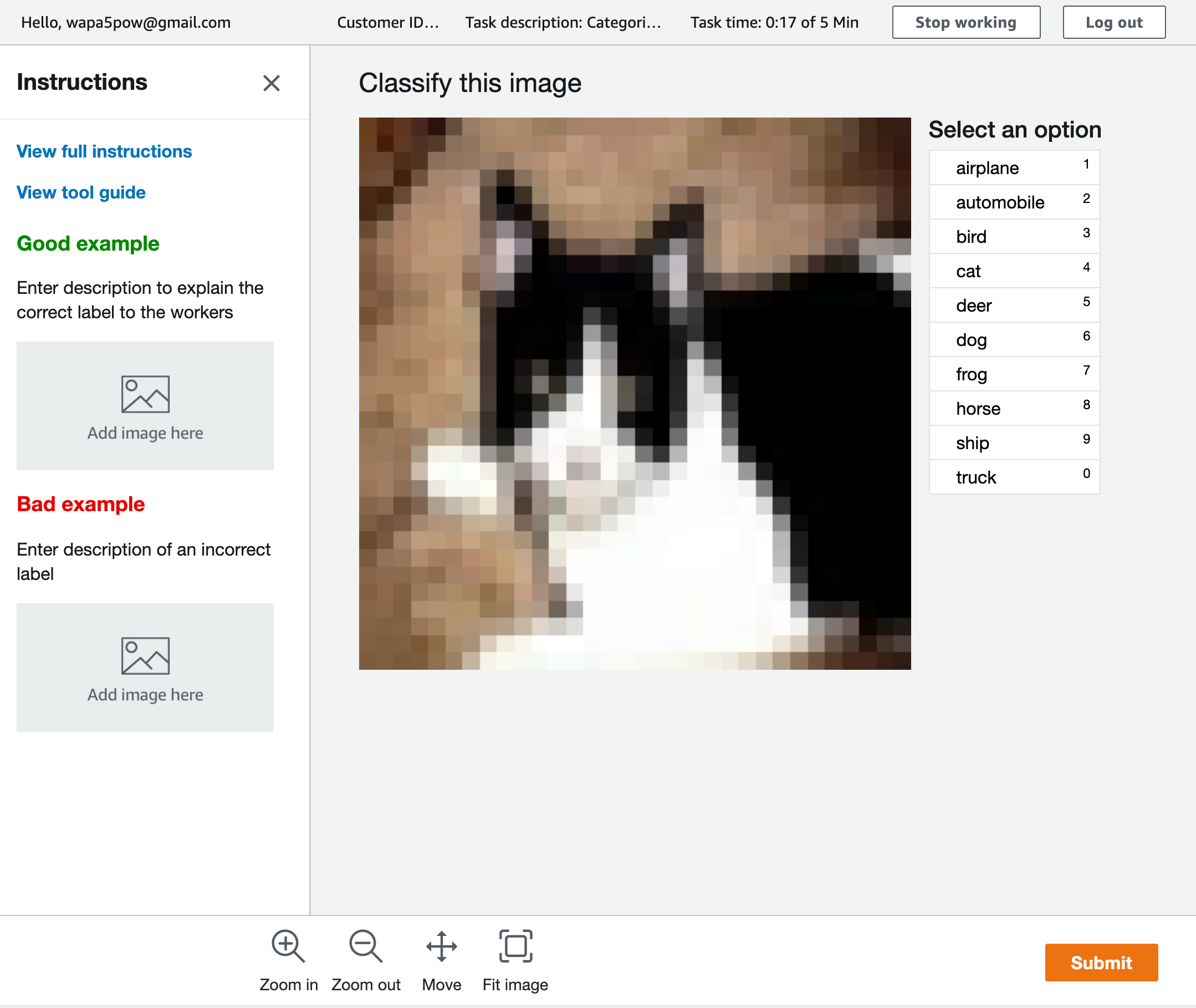
Ground Truth > ラベリングジョブからジョブを作ります。Ground TruthはS3の特定フォルダ(今回ならs3://bucket_name/cifar-10/dataset/ground_truthです)にイメージをおいてそれを指定するラベル付け作業者(emailで指定可能)にラベル付けしてもらいます。作業開始のemailが送られるとそこにURL、アカウント名(email)、パスワードがあるのでアクセスします。以下のような感じでラベル付けしていきます。
作業者のラベル付けするWebページは以下のような感じです。
すべての作業者のラベル付けが終わると1つのラベルに付き以下のようなJSONが出力されます。
{
  "source-ref": "s3://bucket_name/cifar-10/dataset/ground_truth/trucking_rig_s_001486.png",
  "cifar-10": 0,
  "cifar-10-metadata": {
    "confidence": 0.92,
    "job-name": "labeling-job/cifar-10",
    "class-name": "truck",
    "human-annotated": "yes",
    "creation-date": "2019-10-13T22:55:30.029703",
    "type": "groundtruth/image-classification"
  }
}
モデル構築時は以下のようなフォルダ構成にしたいので、自分で用意したデータセットの場合はGround Truthの結果をPythonなどスクリプトを使って指定のフォルダ構成にします。
├── train
|   ├── class_1
|   │   ├── image_train_1_1.png
|   │   ├── image_train_1_2.png
|   │   ...
|   |   └── image_train_xxx.png
|   ├── class_2
|   │   ├── image_train_2_1.png
|   ...
└── test
    ├── class_1
    │   ├── image_test_1_1.png
    │   ├── image_test_1_2.png
    │   ...
    |   └── image_test_xxx.png
    ├── class_2
    │   ├── image_test_2_1.png
今回はすでにラベル付けされているデータセットでCIFAR-10をPNGイメージとして保存した際に上記のフォルダ構成で保存するようにしているのでノートブックで以下を実行するとS3に指定のフォルダの構成を保ってアップロードできます。
for label in label_names:
    for kind in ['train', 'test']:
        !aws s3 cp --recursive dataset/$kind/$label s3://bucket_name/cifar-10/dataset/$kind/$label
ノートブックでKerasを使ったモデルの構築しトレーニングジョブとして実行する
S3に訓練するためのイメージをアップロードできたのでモデルを構築していきます。モデルを構築するには2つの方法があります。
- ノートブック上で訓練する
- SageMakerのトレーニングジョブを利用し、ノートブックとは別インスタンスで訓練させる
1は、ノートブック上で訓練できるのでmodel.fitの訓練経過も変数に入れてすぐにグラフ化できて便利ですが、デープラーニングなど重い処理は、インスタンスタイプによって訓練に時間がかかります。
2で、別インスタンスで訓練するためには訓練内容を別のPythonスクリプトにしなければならないのと出力を変数に入れられないのでファイルに保存してから利用しなければならないので面倒なのですが、訓練している時間だけGPUつきの早いインスタンスを使え訓練時間とお金を節約できるので時間のかかる訓練をする場合はこちらがおすすめです。
今回は実践を想定して2で訓練します。まず以下のような訓練するためのPythonスクリプトをcifar-10-cnn.pyとして保存します。このコードはKerasのサンプルを参考にしています。
from __future__ import print_function

import argparse
import os
import json

import tensorflow as tf
from keras import backend as K
from keras import layers
from keras import models
from keras import optimizers
from keras.preprocessing.image import ImageDataGenerator


def save(model, model_dir):
    sess = K.get_session()
    tf.saved_model.simple_save(
        sess,
        os.path.join(model_dir, 'model/1'),
        inputs={'inputs': model.input},
        outputs={t.name: t for t in model.outputs})


def save_history(history, history_dir):
    with open(os.path.join(history_dir, 'cnn_history.json'), 'w') as f:
        json.dump(history.history, f)


def train(args):
    width = 32
    height = 32
    batch_size = args.batch_size
    epochs = args.epochs
    base_dir = args.train
    train_dir = os.path.join(base_dir, 'train')
    validation_dir = os.path.join(base_dir, 'test')

    category_num = len(os.listdir(train_dir))

    model = models.Sequential()
    model.add(layers.Conv2D(32, (3, 3), padding='same', activation='relu', input_shape=(width, height, 3)))
    model.add(layers.Conv2D(32, (3, 3), activation='relu'))
    model.add(layers.MaxPooling2D((2, 2)))
    model.add(layers.Dropout(0.25))

    model.add(layers.Conv2D(64, (3, 3), activation='relu'))
    model.add(layers.Conv2D(64, (3, 3), activation='relu'))
    model.add(layers.MaxPooling2D((2, 2)))
    model.add(layers.Dropout(0.25))

    model.add(layers.Flatten())
    model.add(layers.Dense(512, activation='relu'))
    model.add(layers.Dense(category_num, activation='softmax'))

    print(model.summary())

    model.compile(loss='categorical_crossentropy',
                  optimizer=optimizers.RMSprop(lr=1e-4),
                  metrics=['acc'])

    train_datagen = ImageDataGenerator(rescale=1./255)
    validation_datagen = ImageDataGenerator(rescale=1./255)

    train_generator = train_datagen.flow_from_directory(
        train_dir,
        target_size=(width, height),
        batch_size=batch_size,
        class_mode='categorical'
    )

    validation_generator = validation_datagen.flow_from_directory(
        validation_dir,
        target_size=(width, height),
        batch_size=batch_size,
        class_mode='categorical'
    )

    # 推論結果のインデックスと対応するクラスを出力
    print(train_generator.class_indices.items())

    history = model.fit_generator(train_generator,
                                  steps_per_epoch=100,
                                  epochs=epochs,
                                  validation_data=validation_generator,
                                  validation_steps=50)
    save_history(history, args.model_dir)
    save(model, args.model_dir)


if __name__ == '__main__':
    parser = argparse.ArgumentParser()

    # hyperparameters sent by the client are passed as command-line arguments to the script
    parser.add_argument('--epochs', type=int, default=12)
    parser.add_argument('--batch-size', type=int, default=128)

    # input data and model directories
    parser.add_argument('--model-dir', type=str, default=os.environ['SM_MODEL_DIR'])
    parser.add_argument('--train', type=str, default=os.environ['SM_CHANNEL_TRAINING'])

    args, _ = parser.parse_known_args()
    train(args)
次にノートブック上で以下を実行します。CIFAR-10イメージをCNNで30エポック訓練します。
import os
import keras
import numpy as np
import sagemaker

sagemaker_session = sagemaker.Session()
bucket_name = sagemaker_session.default_bucket()
input_data = "s3://bucket_name/cifar-10/dataset"

from sagemaker.tensorflow import TensorFlow
from sagemaker import get_execution_role

role = get_execution_role()
estimator = TensorFlow(
    entry_point = "./cifar-10-cnn.py",
    role=role,
    train_instance_count=1,
    train_instance_type="ml.p3.2xlarge",
    framework_version="1.14.0",
    py_version='py3',
    script_mode=True,
    hyperparameters={'epochs': 30, 'batch-size': 32})

estimator.fit(input_data)
訓練がおわったら結果をグラフでみてみます。まずhistoryの結果を訓練結果が保存してあるS3から取得します。
output_dir = estimator.model_dir.replace("/model", "/output")
!mkdir -p tmp
!rm -rf tmp/*
!aws s3 cp --recursive $output_dir tmp/
! cd tmp && tar -xvf "model.tar.gz"

import json
f = open('tmp/cnn_history.json', 'r')
history = json.load(f)
f.close()
ヒストリーから精度と損失をグラフ化します。
import matplotlib.pyplot as plt

acc = history['acc']
val_acc = history['val_acc']
loss = history['loss']
val_loss = history['val_loss']

epochs = range(len(acc))

plt.plot(epochs, acc, 'bo', label='Training acc')
plt.plot(epochs, val_acc, 'b', label='Validation acc')
plt.title('Training and validation accuracy')
plt.legend()
plt.figure()

# 損失値をプロット
plt.plot(epochs, loss, 'bo', label='Training loss')
plt.plot(epochs, val_loss, 'b', label='Validation loss')
plt.title('Training and validation loss')
plt.legend()

plt.show()
出力されたグラフです。
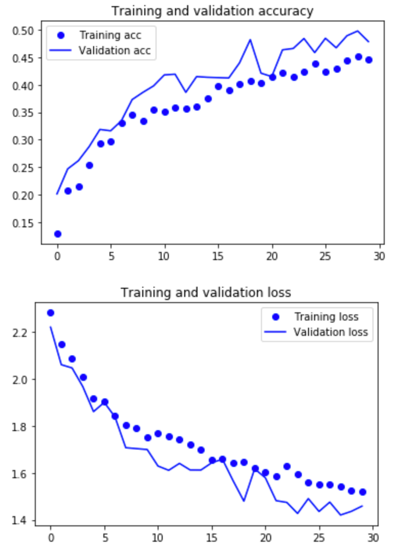
精度は45%前後と低く調整の余地がありますがひとまずこちらですすめます。
推論のエンドポイントを作成し、boto3から呼び出す
モデルができたの推論できるようにします。さきほどのノートブックで以下を実行するだけで推論のインスタンスがデプロイされます。
predicator = estimator.deploy(instance_type='ml.m5.xlarge', initial_instance_count=1)
predicatorを使って推論する
import numpy as np
import matplotlib.pyplot as plt
from PIL import Image

image = Image.open('dataset/ground_truth/dawn_horse_s_000709.png')

# イメージを表示
plt.imshow(image)
plt.show()

# 推論
prediction = predicator.predict(pix.reshape(1, 32, 32, 3))['predictions']
prediction = np.array(prediction)
predicted_label = prediction.argmax(axis=1)
print('The predicted labels are: {}'.format(predicted_label))
結果は7とでました。7はhourseなのでこのイメージの場合は正解です。
boto3で推論する
import boto3
import json
import numpy as np
from PIL import Image

runtime= boto3.client('runtime.sagemaker')
endpoint_name = "tensorflow-training-2019-10-14-02-09-37-730"

image = Image.open('dataset/ground_truth/dawn_horse_s_000709.png')
image_array = np.asarray(image.resize((32,32)))
image_array = image_array.reshape((1,) + image_array.shape)

response = runtime.invoke_endpoint(
    EndpointName=endpoint_name,
    ContentType='application/json',
    Body=json.dumps(image_array.tolist()))

result = json.loads(response['Body'].read())
np.argmax(result['predictions'][0])
こちらも結果は7となりました。ちゃんと呼び出せてそうです。なお、image_array.shapeを確認すると(1, 32, 32, 3)なのでリクエストのJSONには[75, 94, 50]のような色の情報をもった1x32x32の配列が格納されています。
まとめ
SageMakerを使ってイメージ分類を、ラベル付け・訓練・推論まで一通り実行してみました。初めてさわると覚えることが多いのですが、一通りやってみるとSageMakerの可能性が感じられました。特にローカルのPCで訓練していたときはすごく時間がかかっていたものがSageMakerのとレージングジョブを使うと、数倍〜数十倍はやくなるのでイテレーションが早く回せます。
実践で使っていくには、ハイパーパラメータ調整・ノートブックファイルのGit化など他にもやることがありますがこれからSageMakerをたくさん触っていくのが楽しみです。